Tutorial

This section shows a basic usage-example and thus introduces the main concepts of Pylocator. It is arranged as a step-by-step instruction and uses a dataset which is available here: post2std_brain.nii.gz.

Loading the MR image

After starting the program (refer to Installation for details) you’ll first see a dialog prompting for a Nifti-file. Choose the “post2std_brain.nii.gz” file, downloaded from above.

Note

The MR image is a post-implantation image containing two temporal depth electrodes, temporo-lateral strip electrodes and temporo-basal electrodes on either side.

It was preprocessed using FSL:

1. first, a pre-implantation image was brain-extracted and normalized to a MNI152_T1_1mm-template. The transformation matrix was saved.
2. then the post-implantaion image was normalized to the pre-implantation image, also saving the matrix
3. these two matrices were then concatenated; using this new matrix the post-implantation image was transformed to the MNI template.
4. finally, the image was brain-extracted.

Then the MRI is loaded and the main window of PyLocator pops up. It consists of two toolbars (a main toolbar at the top and a secondary at the left side) and 5 subwindows. Four of these windows come to live immediately..

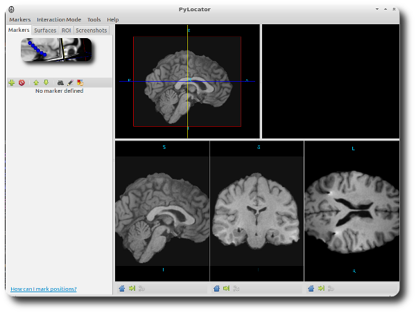
The lower row shows three slice views of the MR volume (let’s call them slice widgets from now on). Exactly the same cut planes are also visible in the upper-left subwindow (subsequently called planes widget), but arranged in a 3d setting.

Controlling the views

Getting used to interacting with these widgets is maybe the hardest time using PyLocator. It’s typical VTK style: you’ll need all three mouse buttons and your keyboard, and their respective behaviour depends on where you use them. But just go ahead and try, once you get a feeling, it works like a charm.

While you’re in “Interact Mode” (button Enable Interact in the left toolbar, default), the controls basically are:

Planes widget

Left mouse button

When clicked on one of the planes, the corresponding coordinates and intensity are displayed. If you drag this button somewhere not on any plane, you can rotate the virtual camera around the planes object. If you additionally hold down the Ctrl-Key, the camera will roll around its viewing direction.

Right mouse button

When dragged on-plane, you can adjust the thresholds of the colormap for all planes. Drag left/right for adjusting the level (center of the colormap-range), drag up/down to change the window (width of the colormap-range). To clarify this concept, let’s look at a little “diagram”:

                           _______white___________
                          /
                         /
                        /
                       /
                      /
_____black___________/
                     |  ^  |    Level
                     <----->    Window

When dragged off-plane, you can move your camera into / out of the scene.

Middle mouse button

When dragging on-plane you can move the planes. Dragging at the edges rotates the plane. Off-plane you can translate the focal point of the camera.

Slice widgets

These slices are automatically synchronized to the cut planes in the planes widget. The right and middle mouse button behave mailny the same as off-plane in the plane widget. Additionally, you can use the mouse wheel to slowly move the slices back and forth.

Marking electrodes

PyLocator uses Markers to help in the localization of electrodes. Every Marker is represented as a small sphere in 3d-space. In the plane widget you can see these spheres, while in the slice widgets they are visible as small circles (if the slice intersects the sphere).

Inserting markers

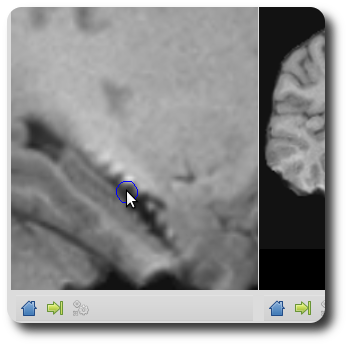
First, move the cut planes so that you can see the electrode you want to mark. Use the controls as described above to zoom in. Move you mouse above the electrode location (in one of the slice widgets) and press the button I (as in insert) on your keyboard. A blue circle appears,

Congratulations! You just inserted your first electrode marker.

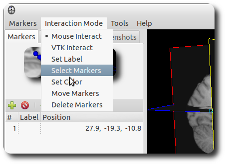
If you aren’t satisfied with it’s location, use the Interaction Menu to swtich to the “Move Marker” tool to adjust it.

You might have noticed that after inserting markers, also the fifth subwindow isn’t empty anymore. You can see the little spheres also there. Let’s call it the surface widget. We will explain it later.

Labeling the markers

After having marked some electrodes, you can assign labels to the electrodes. Use the corresponding mode from the interaction menu, and the click on one of the spheres in the plane widget or one of the circles in the slice widgets.

A little dialogue will pop up, you can enter a label, hit O.k. Afterwards, the label shows up as yellow text next to the marker.

You can reedit the labels anytime later using the same method.

Alternatively, oyu can select the marker to label from the markers list. Click on the corresponding toolbar button and the same dialog will appear.

We use some regex-matching to guess the next electrode name, so after labeling one electrode “TL01”, for the next electrode PyLocator will propose “TL02”.

Saving markers to file

Finally, when you want to export the electrode locations, you can save them as a simple text file to disk. Use the Save to-entry from the Markers menu. Choose a directory and filename and your done.

electrode_locations.txt:

TBPR1,22.3044795975,-5.109097651,-37.8967504764,3.0,0.0,0.0,1.0
TBPR2,31.4296973957,-10.476872826,-37.8967504764,3.0,0.0,0.0,1.0
TBPR3,40.0181376763,-16.918203037,-37.8967504764,3.0,0.0,0.0,1.0
TBPR4,49.1433554745,-22.82275573,-37.8967504764,3.0,0.0,0.0,1.0
TL01,-25.062664026,-6.375814565,-29.9888764281,3.0,0.0,0.0,1.0
TL02,-25.632289616,-10.015602878,-26.9951491745,3.0,0.0,0.0,1.0
TL03,-26.63892536,-13.301689266,-23.680670446,3.0,0.0,0.0,1.0
TL04,-27.604637459,-17.54492081,-20.3931495947,3.0,0.0,0.0,1.0
TL05,-28.415850937,-21.109297964,-17.1291834355,3.0,0.0,0.0,1.0
...

The first column contains the labels you assigned to the markers, the next three columns are the indices / coordinates. Columns 5 to 8 can be ignored, they contain the marker size and its color.

Note

In v0.1 of PyLocator, the affine transformation was not applied for visualization. It was rather used at save time to create a second file. If you decided to use “electrode_locations.txt”, the file “electrode_locations.txt.conv” used to be created in the directory. While the first one contained the voxel-indices where the marks were set (as floats, due to interpolation) the second one had the coordinates in scanner space [1] as obtained by the affine transform stored in the Nifti file.

Here is an example how the old files might have looked like:

electrode_locations.txt:

TBPR1,67.6955204025,120.890902349,34.1032495236,3.0,0.0,0.0,1.0
TBPR2,58.5703026043,115.523127174,34.1032495236,3.0,0.0,0.0,1.0
TBPR3,49.9818623237,109.081796963,34.1032495236,3.0,0.0,0.0,1.0
TBPR4,40.8566445255,103.17724427,34.1032495236,3.0,0.0,0.0,1.0
TL01,115.062664026,119.624185435,42.0111235719,3.0,0.0,0.0,1.0
TL02,115.632289616,115.984397122,45.0048508255,3.0,0.0,0.0,1.0
TL03,116.63892536,112.698310734,48.319329554,3.0,0.0,0.0,1.0
TL04,117.604637459,108.45507919,51.6068504053,3.0,0.0,0.0,1.0
TL05,118.415850937,104.890702036,54.8708165645,3.0,0.0,0.0,1.0
...

If you reload the same image again sometime later, you can also load these files back into the program to recover all markers. You can also use the locations in other programs, e.g., your own analysis scripts. Althoug reading csv-files is really easy in Python, we offer anobject-oriented API to simplify access to the electrode file. See module pylocator.misc.

Note

When loading markers from disk, be careful with old files: if they were created with PyLocator version < 0.2, do choose the .conv-file. Otherwise the locations will be messed up

Rendering 3d-surface

Now let’s move our attention to the upper right subwindow, the surface widget. You already see some electrode markers inside it and can use the same controls as for the planes widget (only setting window/level doesn’t make sense here).

We use this subwindow to render iso-surfaces for our volumetric data. [2] This is especially helpful for locating

1. subdural electrodes, like strips and grids, in brain extracted MR images and
2. surface-electrodes in simultaneous EEG / fMRI experiments.

To create a iso-surface, choose the button “Surface” from the main toolbar. A dialogue shows up where we can make all necessary settings. We have to choose a threshold value for the iso surface. For now, you can accept the default value.

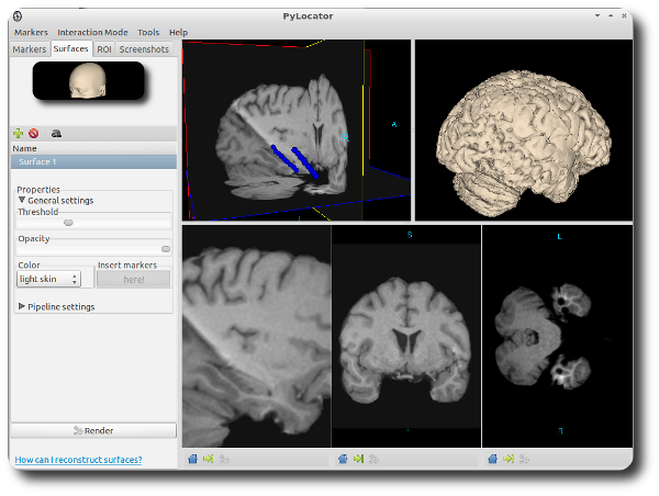
Click on “Add segment” (we could render more than one iso surface, but we won’t do for now) and then “Render”. After a short while, you’ll see your iso surface inside the surface widget. You can see the gyri and sulci and - if you search a little bit - you can find the locations of the subdural electrodes as additional “bumps”.

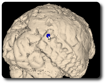
What comes in handy now is that you can insert makers also here just as you can inside the slice widgets: Move the mouse cursor above the “bump” you want to mark and hit I. Another little sphere appears, just at the point on the surface you were pointing at.

Again, you can correct the marker locations within the slice widgets, label them in the planes widget or one of the slice widgets, and finally save all markers to disc.

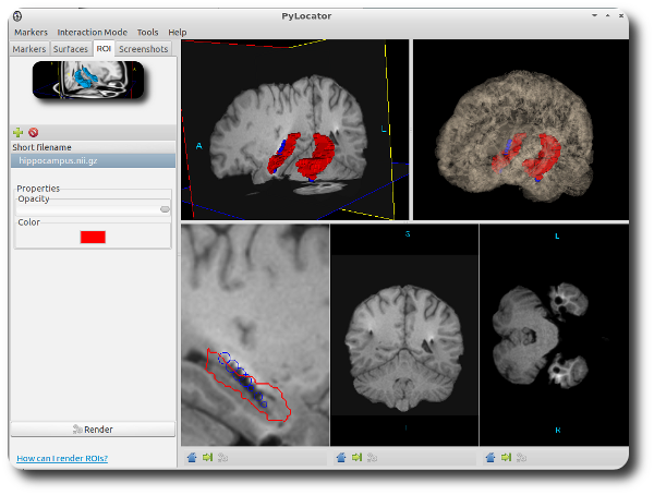
Rendering ROIs

To give a better orientation while surfing throw brain structures it might be helpful to show some regions-of-interest in your visualization. You can load binary Nifti files, i.e., images with only intensity values of 0 and 1, as ROIs. For more information, see How can I render regions-of-interest?

Taking screenshots

A feature recently added to PyLocator is its ability to take screenshots of the 3d-widgets. In contrast to using an external program for doing so, we can achieve a higher quality using VTK.

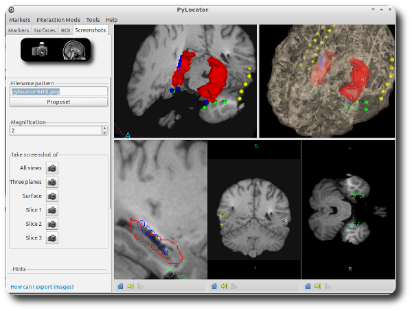
Click on the button “Screenshot” in the main toolbar. A dialog appears (see above). Here, you can pick a filename pattern (it is important to keep the %03i within the pattern, as an automatically incremented counter is added here). You can also have a pattern proposed by PyLocator, is will be based on the name of the MRI Nifti file.

Next, choose your desired magnification. The currently rendered images in each widget will be resampled accordingly by VTK, resulting in a higher resolution than a-posteriori resizing a normal screenshot.

You can use the buttons in the dialog to take photos of individual widgets or of all widgets.

Footnotes

[1]	If you normalized the MRI image to some standard brain (the tutorial file is normalized to MNI152, T1, 1mm voxel size) these coordinates where in standard space, e.g. MNI coordinates

[2]	Iso surfaces are the 3d analogy to contour plots.